Factors in R
Load needed packages
pacman::p_load(forcats,ggplot2,tidyverse,lubridate)
Reorder Levels
| Goal | forcats function |
|---|---|
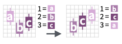
| Set order manually | fct_relevel(f, 'b', 'a','c') |
| Set order based on another vector | fct_reorder(f, x) |
| Set order based on which category is most frequent | fct_infreq(f) |
| Set order based on when they first appear | fct_inorder(f) |
| Reverse factor order | fct_rev(f) |
| Rotate order left or right | fct_shift(f, steps) |
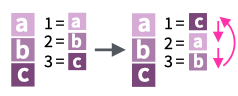
fct_relevel()
- Relevel to the top
f <- factor(letters[1:4])
levels(f)
## [1] "a" "b" "c" "d"
fct_relevel(f, "b", "c")
## [1] a b c d
## Levels: b c a d
- Relevel to the end
fct_relevel(f, "a", after = Inf)
## [1] a b c d
## Levels: b c d a
- Relevel with a function
fct_relevel(f, sort)
## [1] a b c d
## Levels: a b c d
fct_relevel(f, rev)
## [1] a b c d
## Levels: d c b a
fct_inorder()Reorder by first appearance
f <- factor(c("b", "b", "a", "c", "c", "c"))
fct_inorder(f)
## [1] b b a c c c
## Levels: b a c
fct_infreq()reorder by frequency
fct_infreq(f)
## [1] b b a c c c
## Levels: c b a
fct_inseq()reorder by numeric order
f <- factor(1:3, levels = 3:1)
fct_inseq(f)
## [1] 1 2 3
## Levels: 1 2 3
fct_reorder
ggplot(iris, aes(fct_reorder(Species, Sepal.Width), Sepal.Width)) +
  geom_boxplot()

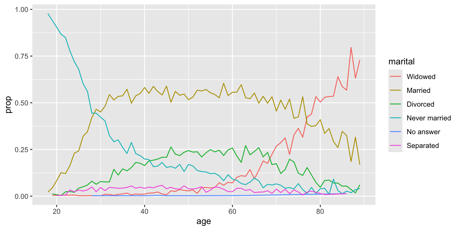
fct_reorder2
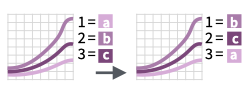
fct_reorder2(factor,x,y)reorders the factor by the y values associated with the largest x values.- This makes the plot easier to read because the line colours line up with the legend.
- Noticed the legend order aligns with the line plot sequence at its endpoint.
by_age <- gss_cat %>%
  filter(!is.na(age)) %>%
  count(age, marital) %>%
  group_by(age) %>%
  mutate(prop = n / sum(n))
ggplot(by_age, aes(age, prop, colour = fct_reorder2(marital, age, prop))) +
  geom_line() +
  labs(colour = "marital")
fct_rev()
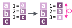
f <- factor(letters[1:4],levels=letters[c(3:4,1:2)])
levels(f)
## [1] "c" "d" "a" "b"
f%>%fct_rev()
## [1] a b c d
## Levels: b a d c
fct_shift()
x<-wday(seq(ymd("2024/1/1"), ymd("2024/1/7"), by = "1 day"), label = TRUE, week_start = 1)
x
## [1] Mon Tue Wed Thu Fri Sat Sun
## Levels: Mon < Tue < Wed < Thu < Fri < Sat < Sun
fct_shift(x,-1)
## [1] Mon Tue Wed Thu Fri Sat Sun
## Levels: Sun < Mon < Tue < Wed < Thu < Fri < Sat
Edit Factor Labels
| Goal | forcats function |
|---|---|
| Manually change the label(s) | fct_recode(f, new_label = "old_label") |
| Systematically change all labels | fct_relabel(f, function) |
fct_recode
x <- factor(c("apple", "bear", "banana", "dear"))
fct_recode(x, fruit = "apple", fruit = "banana")
## [1] fruit bear  fruit dear
## Levels: fruit bear dear
fct_relabel
iris$Species%>%fct_relabel(stringr::str_to_upper)%>%table()
## .
##     SETOSA VERSICOLOR  VIRGINICA
##         50         50         50
Collapse or lump Levels
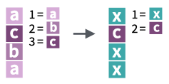
fct_collapse
x<-wday(seq(ymd("2024/1/1"), ymd("2024/1/7"), by = "1 day"), label = TRUE, week_start = 1)
x
## [1] Mon Tue Wed Thu Fri Sat Sun
## Levels: Mon < Tue < Wed < Thu < Fri < Sat < Sun
lvl=levels(x)
fct_collapse(x,weekdays=lvl[1:5],weekends=lvl[6:7])
## [1] weekdays weekdays weekdays weekdays weekdays weekends weekends
## Levels: weekdays < weekends
fct_lump
fct_lump_min(): Lumps levels that appear fewer thanmintimes.
x <- factor(rep(LETTERS[1:9], times = c(40, 10, 5, 27, 1, 1, 1, 1, 1)))
x %>%
  fct_lump_min(5) %>%
  table()
## .
##     A     B     C     D Other
##    40    10     5    27     5
fct_lump_prop(): Lumps levels that appear in fewer than (or equal to)prop * ntimes.
x %>%
  fct_lump_prop(0.10) %>%
  table()
## .
##     A     B     D Other
##    40    10    27    10
fct_lump_n(): Lumps all levels except for thenmost frequent (or least frequent ifn < 0).
x %>%
  fct_lump_n(3) %>%
  table()
## .
##     A     B     D Other
##    40    10    27    10
fct_lump_lowfreq(): Lumps together the least frequent levels, ensuring that “other” is still the smallest.
x %>%
  fct_lump_lowfreq() %>%
  table()
## .
##     A     D Other
##    40    27    20
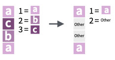
fct_other()
fct_other(): Manually replace levels with “other”
x%>%fct_other(keep = c("A", "B"))%>%table()
## .
##     A     B Other
##    40    10    37
x%>%fct_other(drop = c("A", "B"))%>%table()
## .
##     C     D     E     F     G     H     I Other
##     5    27     1     1     1     1     1    50
Add or Subtract Levels
fct_expand
f <- factor(letters[1:3])
fct_expand(f, "d", "e", "f")
## [1] a b c
## Levels: a b c d e f
fct_drop
f <- factor(c("a", "b"), levels = c("a", "b", "c"))
f%>%fct_drop()
## [1] a b
## Levels: a b